Digital Twin-Driven Safety Protocol Development for HRI in German Retail Stores - Part 2

In Part 1, we explored foundational technologies for developing safety protocols and compliance mechanisms in retail robotics, including simulation environments like Gazebo and NVIDIA Isaac Sim, and key safety standards such as ISO 13482. Building upon that groundwork, Part 2 focuses on testing the practical implementation of these protocols within Gazebo Classic, specifically examining how different combinations of planners and controllers influence robot behavior in various scenarios. This analysis provides actionable insights into achieving safe, efficient navigation in dynamic retail environments.

Understanding Robot Decision-Making: Local and Global Planners

Now that we have discussed the need to validate safety protocols and data protection policies—and identified each—it is time to explore what makes a robot autonomous. Specifically, we will dive into how robots make decisions in different scenarios and how planners influence these decisions during operation.

Local and Global Planners

Robots rely on two types of planners to navigate their environments: local planners and global planners. Each plays a distinct role in ensuring safe, efficient, and autonomous operation.

Aspect	Local Planner	Global Planner
Scope	Handles short-term, real-time navigation and obstacle avoidance.	Plans long-term paths from the robot’s start point to its goal.
Focus	Dynamic obstacle handling and maintaining a smooth, collision-free trajectory.	Optimizing the overall route based on the map, environment, and defined goals.
Frequency	Operates at a higher frequency (e.g., 10 Hz) for real-time adjustments.	Operates at a lower frequency (e.g., 1 Hz) to minimize computational overhead.
Impact on Safety	Ensures immediate responsiveness to nearby obstacles and path deviations.	Avoids hazardous routes or areas that could compromise the robot's operation.
Key Parameters	Velocity limits, inflation radius, yaw tolerance for precise control.	Map cost layers, goal tolerance for efficient and safe long-term planning.

Nav2 Global Planners and Local Controllers

The Nav2 stack provides a robust framework for implementing local and global planners, each tailored to specific use cases and operational environments. The table below categorizes the available planners and controllers:

Type	Name	Description
Global Planner	NavFn Planner	Utilizes Dijkstra's algorithm to compute the shortest path on a costmap.
Global Planner	Smac Planner	Offers different variants, including 2D and Hybrid-A* planners, suitable for various robot types and environments.
Global Planner	Theta Planner	Computes paths that are more direct by allowing diagonal movements, reducing unnecessary turns.
Local Controller	DWB (Dynamic Window Approach)	Evaluates a set of possible trajectories and selects the one that optimally balances progress toward the goal, speed, and obstacle avoidance.
Local Controller	Regulated Pure Pursuit	Focuses on following the global path accurately, adjusting the robot's speed based on proximity to obstacles and path curvature.
Local Controller	MPPI (Model Predictive Path Integral)	Uses a model predictive control approach to optimize control commands over a future horizon, considering the robot's dynamics and environmental constraints.
Local Controller	Rotation Shim Controller	Handles in-place rotation behaviors, ensuring the robot can correctly orient itself before proceeding along the path.

Moving Forward

In the following sections, we will explore how these planners influence robot behavior in specific scenarios:

1. Going in a Straight Line
2. Navigating Around Static Obstacles
3. Navigating Around Dynamic Obstacles

Relevant Parameters for Navigation Experiments

These are the default parameters of the Nav2 stack. In the following experiments, these parameters will be tweaked for different scenarios, planners, and controllers:

Parameter Group	Parameter Name	Value	Purpose/Description
AMCL Configuration	use_sim_time	True	Ensures simulation time is used for synchronization.
Controller Server	controller_frequency	20.0	Frequency at which local controllers compute control commands.
Costmap Parameters	local_costmap.width	3.0	Defines the width of the local costmap in meters.

Combination 1: NavFn Planner + DWB Local Planner

This configuration employs the NavFn Planner for global path planning and the DWB Local Planner for local trajectory adjustments.

Component	Plugin/Server	Type	Description
Planner Server	nav2_navfn_planner/NavfnPlanner	Global Planner	Computes the shortest path from start to goal using Dijkstra's algorithm on a costmap.
Controller Server	dwb_core::DWBLocalPlanner	Local Controller	Evaluates possible trajectories and selects the one that optimally balances progress, speed, and obstacle avoidance.

Observations and Results

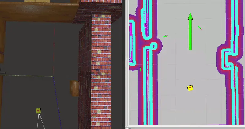
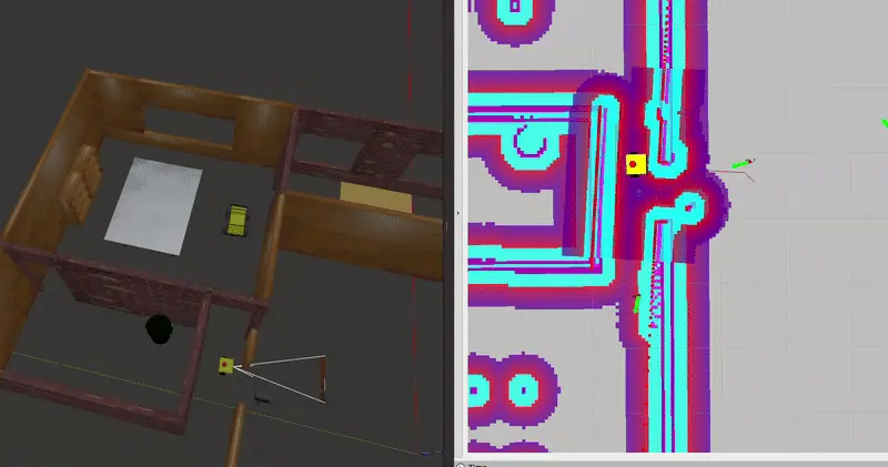
1. Straight-Line Movement
   
   • The robot adhered closely to the planned trajectory with minimal drift.
   • Smooth motion was achieved by tuning parameters such as max_velocity and yaw_goal_tolerance.
   
   Note: The scene is speed-forwarded and does not reflect true speed (i.e., 0.26 m/s).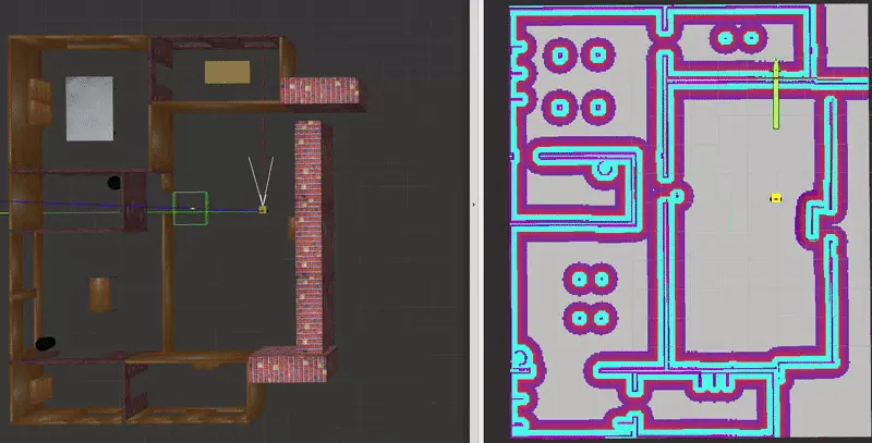
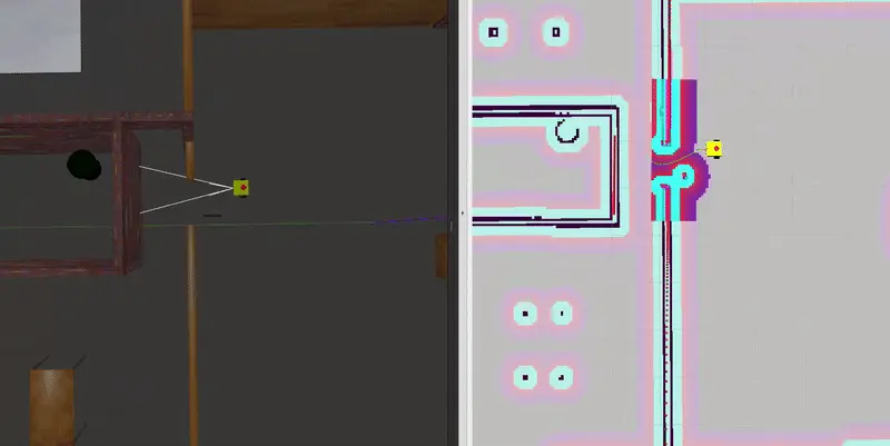
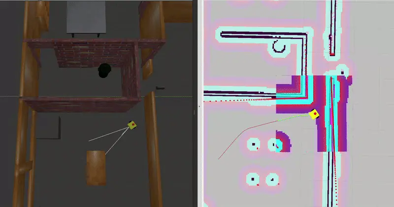
2. Static Obstacles
   
   • The robot slowed down at the junction and adjusted its speed.
   • Trajectory adjustments were made by the robot, and it remained on the global path.
   • Minor path deviations were corrected by the local controller.
   
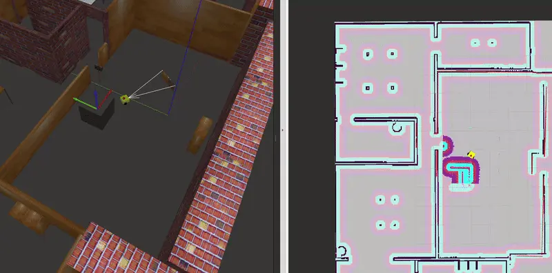
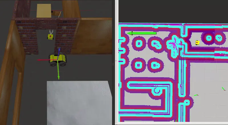
3. Dynamic Obstacles
   
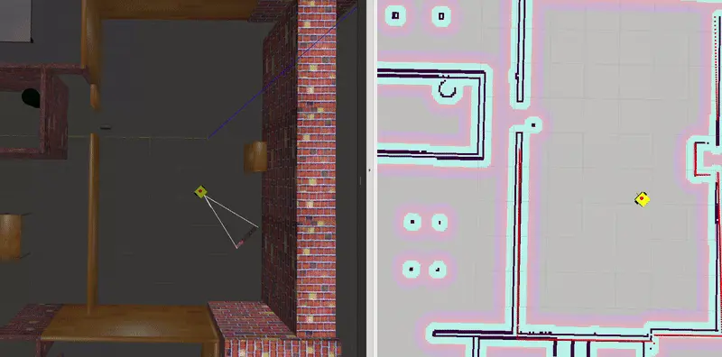
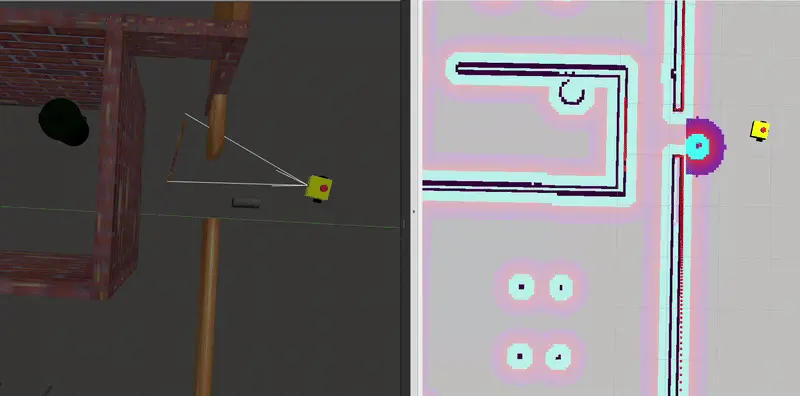
   • The robot successfully responded to a moving cube as a placeholder for a moving person but exhibited slight delays when encountering faster objects.
   • The robot did not collide with the moving cube.
   • The robot did not maintain a safe distance, likely due to suboptimal tuning of parameters such as inflation_radius, PathDist.scale, or obstacle_max_range in the local and global costmaps.
   

Performance Summary

Scenario	Performance
Straight-Line Movement	Smooth and precise navigation.
Static Obstacles	Reliable obstacle avoidance with minor deviations.
Dynamic Obstacles	Adequate responsiveness to slow-moving obstacles; improvement needed for fast-moving objects and maintaining safe distance.

Future Considerations

• The TEB Local Planner could be explored for enhanced handling of dynamic obstacles.
• The Theta* Global Planner may be utilized for more direct and efficient path generation.

Combination 2: NavFn Planner + MPPI Controller

This configuration utilizes the NavFn Planner for global path planning and the MPPI (Model Predictive Path Integral) Controller for local trajectory optimization. This combination is designed to balance efficiency, smoothness, and dynamic obstacle handling.

Why MPPI Controller is a Good Choice

The MPPI Controller is well-suited for dynamic environments requiring real-time adjustments. It optimizes trajectories by considering the robot’s dynamics and environmental constraints, making it highly effective for:

• Dynamic Obstacle Avoidance: Evaluates multiple trajectories to select the optimal path while avoiding collisions.
• Smooth Path Generation: Produces jerk-free motions for stable operations.
• Real-Time Performance: Delivers responsive and efficient control in dynamic scenarios.

Relevant Parameters for MPPI Controller

Parameter	Value	Description
time_horizon	1.5	Time horizon over which the trajectory is optimized.
desired_linear_velocity	0.5	Target velocity for the robot's linear motion.
desired_angular_velocity	1.0	Target velocity for the robot's angular motion.
linear_acceleration_limit	2.0	Maximum allowed linear acceleration for smoother motion.
angular_acceleration_limit	3.0	Maximum allowed angular acceleration for smoother turns.
optimizer_iterations	1000	Number of iterations for trajectory optimization in each cycle.
cost_weights.path_following	10.0	Weight for staying close to the planned path.
cost_weights.collision_avoidance	15.0	Weight for avoiding collisions with obstacles.
cost_weights.smoothness	5.0	Weight for ensuring smooth trajectories.
lookahead_dist	0.6	Distance ahead of the robot for trajectory optimization.
transform_tolerance	0.1	Tolerance for transform lookups to ensure stability in real-time adjustments.
visualize_optimizer	true	Enables visualization of the optimized trajectories for debugging in RViz.

Testing Scenarios and Observations

1. Straight-Line Movement
   
   • The robot followed a smooth and precise trajectory with minimal drift.
   • Real-time trajectory optimization ensured stable motion.
   
2. Navigating Static Obstacles
   
   • The controller successfully adjusted the robot's path to avoid obstacles, maintaining smooth transitions.
   • Dynamic trajectory optimization minimized unnecessary deviations.
   
3. Navigating Dynamic Obstacles
   
   • The robot responded effectively to moving obstacles, recalculating the trajectory in real time.
   • The robot maintained a safe distance from the moving object.
   • Optimized control commands reduced delays in avoiding faster-moving objects.
   

Performance Summary

Scenario	Performance
Straight-Line Movement	Smooth and precise navigation.
Static Obstacles	Reliable obstacle avoidance with smooth trajectory adjustments.
Dynamic Obstacles	Effective real-time responses to moving obstacles.

Conclusion

The combination of NavFn Planner and MPPI Controller provided robust performance across all scenarios. Its ability to handle dynamic obstacles and generate smooth trajectories makes it an excellent choice for complex environments.

Future Improvements

• Further tuning of cost weights and time horizon could enhance responsiveness in highly dynamic settings.
• Exploring alternate global planners, such as Smac (Hybrid-A*), may yield better path efficiency for intricate environments.

Combination 3: NavFn Planner + Regulated Pure Pursuit Controller

This configuration utilizes the NavFn Planner for global path planning and the Regulated Pure Pursuit Controller for local trajectory adjustments. While this combination is highly efficient for straight-line movements, its performance diminishes when navigating through close proximities or dynamic environments.

Why Regulated Pure Pursuit Controller is a Good Choice

The Regulated Pure Pursuit Controller is known for its simplicity and reliability in following global paths, particularly in open environments. It is designed to scale its velocity based on proximity to obstacles and path curvature, ensuring smooth and precise motion.

• Ideal for Straight-Line Movements: Ensures smooth and predictable navigation without significant path deviations.
• Velocity Regulation: Dynamically adjusts speed to maintain safety when approaching obstacles.
• Ease of Tuning: Fewer parameters compared to more complex controllers, simplifying configuration.

Relevant Parameters for Regulated Pure Pursuit Controller

Parameter	Value	Description
desired_linear_vel	0.5	Target velocity for the robot's linear motion.
lookahead_dist	0.6	Distance ahead of the robot for trajectory adjustments.
min_lookahead_dist	0.3	Minimum distance for trajectory adjustments.
max_lookahead_dist	0.9	Maximum distance for trajectory adjustments.
rotate_to_heading_angular_vel	1.8	Angular velocity for orienting toward the path heading.
use_velocity_scaled_lookahead_dist	false	Disables scaling of lookahead distance based on velocity.
use_collision_detection	true	Enables obstacle detection for safer navigation.
max_allowed_time_to_collision_up_to_carrot	1.0	Maximum allowed time to potential collisions along the path.
min_approach_linear_velocity	0.05	Minimum velocity when approaching a goal or obstacle.
transform_tolerance	0.1	Tolerance for transform lookups to ensure stability in real-time adjustments.

Testing Scenarios and Observations

1. Straight-Line Movement
   
   • The robot navigated smoothly and efficiently, adhering to the global path without significant deviations.
   • Velocity regulation ensured stable and precise motion.
   
2. Navigating Static Obstacles
   
   • Performance was suboptimal, particularly when passing through close gaps.
   • The robot struggled with efficiency compared to other combinations like NavFn + DWB and NavFn + MPPI.
   
3. Navigating Dynamic Obstacles
   
   • The robot managed to replan and avoid moving obstacles, but the response time was slower than other controllers.
   • While it successfully reached the goal pose, the delay in path adjustments indicated limited efficiency in dynamic scenarios.
   

Performance Summary

Scenario	Performance
Straight-Line Movement	Smooth and precise navigation, ideal for open spaces.
Static Obstacles	Struggled with close proximities, less efficient compared to other combinations.
Dynamic Obstacles	Slow in replanning and path adjustments, though able to reach the goal.

Conclusion

The combination of NavFn Planner and Regulated Pure Pursuit Controller is well-suited for open environments with minimal obstacles. However, its limitations become evident in more complex scenarios, such as navigating through tight spaces or reacting to dynamic obstacles.

Future Improvements

• Consider using DWB or MPPI for environments with close proximities or high dynamic activity.
• Fine-tune parameters like lookahead_dist and enable velocity-scaled lookahead for more responsive adjustments.

Interconnected Nodes in Nav2 Stack

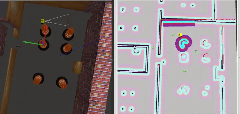
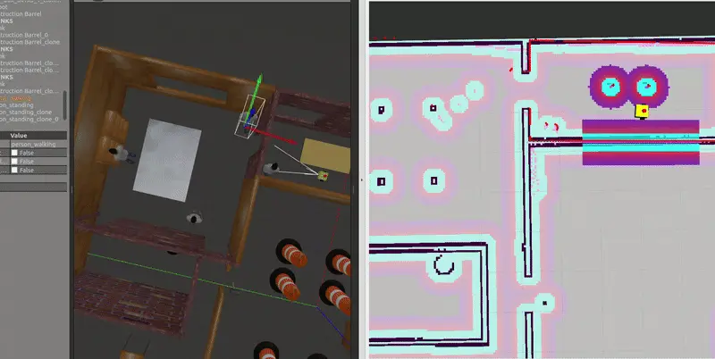
To better understand the communication between various components of the Nav2 stack, here’s the RQT Graph visualization of interconnected nodes. This includes key nodes like the local cost map, global cost map, controller server, planner server, and behavior server.

Note: The RQT graph illustrates how these components interact to ensure smooth and efficient navigation. Each node plays a critical role:

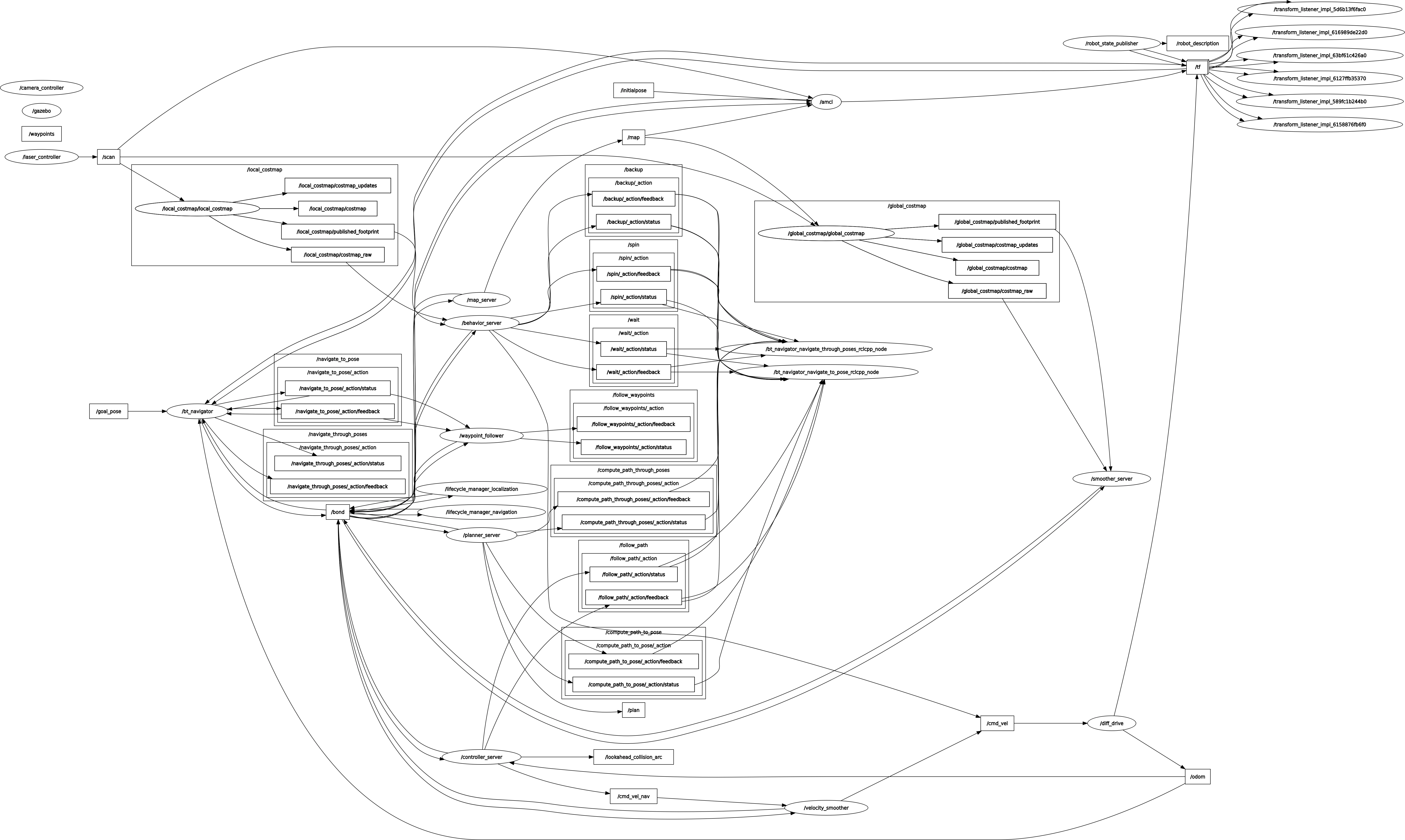
• Planner Server: Computes the global path.
• Controller Server: Adjusts the local trajectory for real-time obstacle avoidance.
• Behavior Server: Manages higher-level behaviors like spinning, backing up, and driving on heading.
• Cost Maps: Provide the environmental representation for planning and obstacle avoidance.

This interconnected structure ensures seamless communication and dynamic adaptability during navigation.

Combination 4: Theta* + Regulated Pure Pursuit Controller

How Theta* Differs from Navfn Planner

The Theta* planner generates any-angle paths with smoother, more direct line segments, while Navfn is constrained to grid-based paths, resulting in more angular and less efficient routes.

Theta* + RPP: Observations and Insights

Straight-Line Movement

In a straightforward scenario, the robot moved along a straight line as expected when the path was unobstructed. This behavior highlights the efficiency of the Theta* planner in generating direct, any-angle paths, reducing unnecessary turns, and optimizing the travel distance.

Static Environment

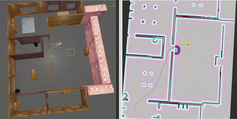
When multiple waypoints were provided, the robot recalculated the path dynamically instead of strictly following the given waypoints. It took a shortcut, reaching the goal faster than if it had adhered to the exact waypoints.

Reason: The Theta* planner is designed to optimize for the shortest and most efficient path between the start and goal. Waypoints, unless enforced as strict constraints, are treated as optional guides. The recalculated shortcut reflects the planner’s inherent focus on path optimization and reduced traversal time.

Dynamic Environment

In a dynamic setup, a walking person primitive was introduced as a moving obstacle:

• First Trial: The robot collided with the moving person, likely due to limitations in the RPP local planner as observed in conjunction with the Navfn planner, which did not react quickly enough to the dynamic change.
• Second Trial: After the person moved aside, the robot successfully stopped, recalculated a shorter path, and reached the goal.

Reason: This outcome underscores the adaptability of Theta* + RPP (Reactive Path Planning). The planner dynamically recalculated the path based on real-time updates, showcasing its ability to handle dynamic obstacles effectively. The successful adjustment in the second trial highlights the importance of robust integration between the global and local planning layers.

Performance Summary

Feature	Performance	Comments
Straight-Line Movement	Smooth and efficient direct paths.	Theta* generates optimal, any-angle paths, making it ideal for open and unconstrained environments.
Static Obstacles	Dynamically recalculates efficient paths.	Bypasses unnecessary waypoints to optimize travel time and distance in static environments.
Dynamic Obstacles	Relies on the local planner for handling dynamic changes effectively.	RPP’s responsiveness impacts success; improvements in local planner integration could enhance reliability.

These observations illustrate the strengths of Theta* + RPP in both static and dynamic scenarios. While the planner excels at optimizing paths, ensuring a robust local planner is critical for managing dynamic obstacles in real-world environments.

Combination 5: Smac Planner + MPPI

Navigation Performance: Testing Smac Planner + MPPI Controller

The combination of the Smac Planner and MPPI Controller represents an advanced setup designed to handle complex navigation scenarios. While the Smac Planner excels at generating smooth, kinematic-aware paths, the MPPI Controller provides real-time trajectory optimization and dynamic obstacle handling.

Testing Scenarios and Observations

1. Straight-Line Movement
   
   • The robot performed satisfactorily, following a smooth and direct path.
   • No significant deviations or delays were observed.
   
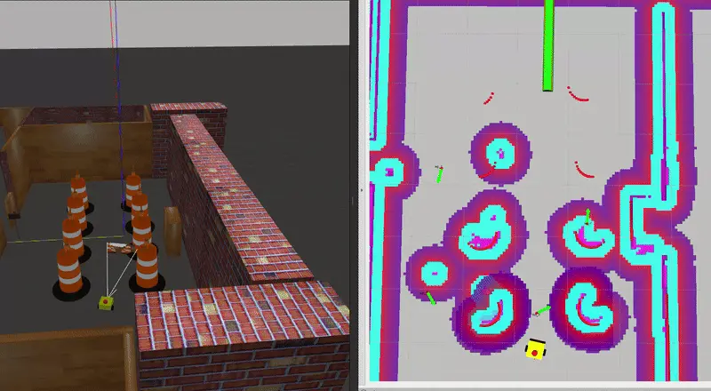
2. Navigating Static Obstacles
   
   • The Smac Planner generated a longer path to avoid obstacles.
   • As the robot approached the goal, it took additional time to stabilize.
   • The robot struggled slightly when passing through narrow gaps between walls, experiencing delays due to repeated replanning.
   
3. Navigating Dynamic Obstacles
   
   • The robot detected a moving wheelchair but was less robust in avoiding it compared to the NavFn + MPPI combination.
   • Multiple replanning attempts were necessary to successfully navigate around the obstacle.
   • Despite these challenges, the robot ultimately reached the goal.
   

Performance Summary

Scenario	Performance
Straight-Line Movement	Smooth and efficient navigation.
Static Obstacles	Planned longer paths; delays in narrow gaps and stabilizing near the goal.
Dynamic Obstacles	Detected moving objects but struggled with robustness; required multiple replans.

Conclusion

The combination of Smac Planner and MPPI Controller demonstrates strong potential for complex environments, particularly in scenarios requiring kinematic awareness and smooth trajectory optimization. However, challenges remain:

• Static Obstacles: Path planning and stabilization need improvement for close proximities.
• Dynamic Obstacles: Responsiveness to fast-moving objects requires further tuning.

Future Improvements

• Optimize Smac Planner parameters for shorter paths and quicker stabilization.
• Fine-tune MPPI cost weights for better responsiveness to dynamic obstacles.

Navigation Performance and Suitability for Safety Scenarios

Global Planner + Local Controller	Straight-Line Movement	Static Obstacles	Dynamic Obstacles	Obstacle Clearance	Dynamic Obstacle Handling
NavFn + DWB	✅	✅	❌	Good	Moderate responsiveness
NavFn + MPPI	✅	✅	✅	Excellent	Highly responsive
NavFn + RPP	✅	❌	❌	Average (struggles in gaps)	Slow
Theta* + RPP	✅	✅	❌	Excellent	Slow
Smac Planner Hybrid + MPPI	✅	✅	❌	Bad	Moderate responsiveness

Key:

• ✅: Suitable
• ❌: Not Suitable
• Obstacle Clearance: Describes the ability to navigate close proximities without collisions (e.g., Excellent, Good, Bad).
• Dynamic Obstacle Handling: Describes the responsiveness to moving obstacles (e.g., Highly responsive, Moderate, Slow).

Important:

Controllers perform differently based on drive types (e.g., differential, Ackermann), impacting navigation results. Proper pairing and tuning are crucial for optimal performance.

Note:

Different drives may give varying results.

Planner Suitability for Different Robot Types

Planner Name	Circular Differential	Circular Omnidirectional	Non-Circular Ackermann	Non-Circular Legged	Non-Circular Differential/Omnidirectional	Arbitrary
NavFn Planner	✅	✅	❌	❌	❌	❌
Smac Planner 2D	✅	✅	❌	❌	❌	❌
Theta* Planner	✅	✅	❌	❌	❌	❌
Smac Hybrid-A* Planner	✅	✅	✅	✅	✅	❌
Smac Lattice Planner	❌	❌	✅	✅	✅	✅

Key:

• ✅: Suitable for this type of robot.
• ❌: Not suitable for this type of robot.

Controller Suitability for Different Robot Types and Tasks

Controller Name	Differential	Omnidirectional	Ackermann	Legged	Primary Task
DWB Controller	✅	✅	❌	❌	Dynamic obstacle avoidance
MPPI Controller	✅	✅	✅	✅	Dynamic obstacle avoidance
RPP Controller	✅	❌	✅	✅	Exact path following
Rotation Shim	✅	✅	❌	❌	Rotate to rough heading
VP Controller	✅	❌	✅	✅	High-speed path tracking

Key:

• ✅: Suitable for this type of robot.
• ❌: Not suitable for this type of robot.

Conclusion

Selecting appropriate planners and controllers is critical for robotic navigation as they must align with the specific task and operational environment. The efficiency of these components varies across different scenarios, such as static and dynamic obstacle navigation, where factors like computational demand, safety, and precision play vital roles. Moreover, tuning parameters in the navigation stack is essential to optimize performance and adaptability. It is, therefore, crucial to comply with safety protocols, especially in environments like retail stores, to ensure safe and efficient human-robot interactions while adhering to regulatory standards and minimizing potential risks.